DistToPiMultilinear

class floulib.DistToPiMultilinear(dist, mode, scale, epsilon)

Bases: Multilinear

This class contains methods to approximate the optimal transformation of unimodal symmetric probability distributions into possibility distributions as multilinear fuzzy subsets.

The optimal transformation of a unimodal symmetric probability distribution is a convex possibility distribution with respect to each side of the mode.The surface under the possibility distribution is also convex. A recursive algorithm can be used to compute a multilinear approximation of the possibility distribution.

Note

DistToPiMultilinear is a subclass of Multilinear, therefore all methods in Multilinear may be used.

Multilinear is a subclass of Plot, therefore all methods in Plot may also be used.

__init__(dist, mode, scale, epsilon)

Constructor

Parameters:

• dist (TYPE) – The probability distribution.

• mode (float) – The mode.

• scale (float) – The scale.

• epsilon (float) – The approximation error.

Return type:

None.

Example

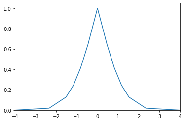
>>> from floulib import DistToPiMultilinear
>>> import numpy as np
>>> from scipy.stats import norm
>>> mean = 0
>>> sigma = 1
>>> normal_dist = norm(mean, sigma)
>>> DistToPiMultilinear(normal_dist, mean, 4*sigma, 0.1).plot()

pi_opt(x=None)

Computes the optimal possibility distribution

Parameters:

x (numpy.ndarray, optional) – The points where the optimal distribution is computed. The default is None.

Returns:

The optimal possibility distribution (as a discrete fuzzy subset if x is not None).

Return type:

DistToPi | Discrete

dpi(x)

Computes the possibility distribution for x.

This method can be used as an interface with other libraries.

Parameters:

x (numpy.ndarray) – The array of points.

Returns:

y – The array of points.

Return type:

numpy.ndarray

Example

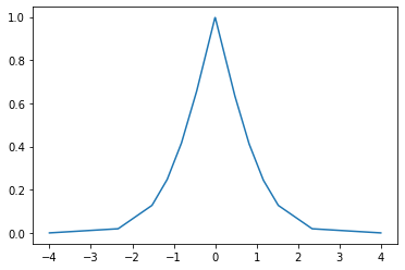
>>> from floulib import DistToPiMultilinear
>>> import numpy as np
>>> from scipy.stats import norm
>>> import matplotlib.pyplot as plt
>>> mean = 0
>>> sigma = 1
>>> normal_dist = norm(mean, sigma)
>>> x = np.linspace(mean - 4*sigma, mean + 4*sigma, 1000)
>>> fig, ax = plt.subplots()
>>> ax.plot(x, DistToPiMultilinear(normal_dist, mean, 4*sigma, 0.1).dpi(x))

print(display='all', format='.3f')

Special method to represent the points of the approximation in human-readable format

Parameters:

• display (str , optional) – If display is ‘left’ or ‘right’, the approximation points for the LHS or the RHS with respect to the mode are displayed. The default is ‘all’.

• format (str, optional) – The format for the display. The default is ‘.3f’.

Return type:

None.

Example

>>> from floulib import DistToPiMultilinear
>>> import numpy as np
>>> from scipy.stats import norm
>>> mean = 0
>>> sigma = 1
>>> normal_dist = norm(mean, sigma)
>>> DistToPiMultilinear(normal_dist, mean, 4*sigma, 0.1).print()
-4.000 0.000
-4.000 0.000
-2.341 0.019
-1.524 0.128
-1.163 0.245
-0.815 0.415
-0.460 0.646
0.000 1.000
0.460 0.646
0.815 0.415
1.163 0.245
1.524 0.128
2.341 0.019
4.000 0.000
4.000 0.000